Branch and bound, branch and cut, branch and price

• 1. Branch-and-Bound
• 2. Branch-and-Cut
• 3. Branch-and-Price

In combination optimization problems and mixed integer programming models, we frequently encounter these three terms: branch-and-bound, branch-and-cut, and branch-and-price. These terms can sometimes be confusing. This blog post aims to summarize them:

1. Branch-and-Bound

Branch-and-bound is the most common method and is covered in the integer programming section of operations research courses in China. Its basic concept is relatively easy to understand and involves three main steps: branching, bounding, and pruning.

For a mixed integer programming problem with the objective of maximization:

• Step 1: Relax the integer constraints, i.e., solve the linear programming problem of the original problem to obtain a solution $\bf x$ with an objective function value that serves as an upper bound for the original problem. Initialize the lower bound of the original problem to negative infinity $-\infty$. (If the linear programming problem has no solution, then the original problem has no solution either)
• Step 2: Termination condition of the algorithm: If there is no direction to branch, then the current lower bound is the optimal solution; otherwise:
• Step 3: Branch: In the solution $\bf x$, select a non-integer decision variable $x_i$ and construct two constraints: one greater than or equal to its ceiling value and one less than its floor value, thus creating two sub-linear programming models.
• Step 4: Bound: Solve the sub-linear programming models. If an integer solution is obtained, it is a feasible solution for the original problem, i.e., a lower bound for the original problem. If it is greater than the current lower bound, update the lower bound; if it is not an integer solution,
  • Step 4.1—Prune: If the sub-linear programming model is infeasible or the obtained solution is smaller than the known lower bound, prune the branch and do not branch further on it.
  • Step 4.2—Continue branching: If the solution to the sub-linear programming problem is greater than the known lower bound, return to step 2 and continue the loop.

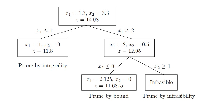
For some simple problems, the steps of branch-and-bound are very intuitive, for example:

2. Branch-and-Cut

The idea of branch-and-cut is to add cutting plane constraints before continuing to branch in step 4.2 of the branch-and-bound process, so that the sub-linear programming problem obtains a smaller solution, i.e., a tighter upper bound for the original problem.

3. Branch-and-Price

In column generation algorithms, when combined with branch-and-bound, the method is called branch-and-price.