Approximation of power function by exponential function

• 1. \((1+x)^{\alpha}\approx 1+\alpha x\)
• 2. \((1+x)^{\alpha}\approx e^{\alpha x}\)

The power function \((1+x)^\alpha\) can be approximated by the exponential function \(e^{\alpha x}\), and even further approximated as \(1+\alpha x\). This approximation is encountered in the introduction of exponential smoothing methods in a book (Fundamentals of Supply Chain Theory).

1. \((1+x)^{\alpha}\approx 1+\alpha x\)

Expanding \((1+x)^\alpha\) around \(x=0\) using Taylor series, we get

When \(\lvert x\rvert <1\), the terms \(x^2, x^3,\dots\) become smaller. If further \(\lvert\alpha x\rvert \ll 1\) (indicating that \(\lvert\alpha x\rvert\) is sufficiently smaller than 1), the terms on the right side of the equation become increasingly smaller, and we can omit the later terms. Therefore, \((1+x)^{\alpha}\approx 1+\alpha x\).

Although a rigorous proof for these two conditions is not found, it seems reasonable.

2. \((1+x)^{\alpha}\approx e^{\alpha x}\)

This approximation can be obtained through Taylor expansion, as follows:

When \(\lvert x\rvert\) is small, \((1+x)^\alpha\) is close to \(e^{\alpha x}\).

In exponential smoothing methods, the weighted historical demand value at time \(i\) is \(\alpha(1-\alpha)^i\) can be approximated as \(\alpha e^{-\alpha i}\). The following graphs illustrate the degree of approximation for these two functions.

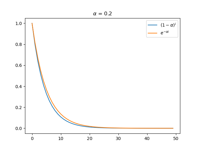
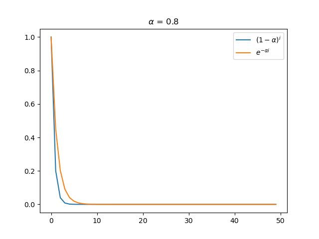
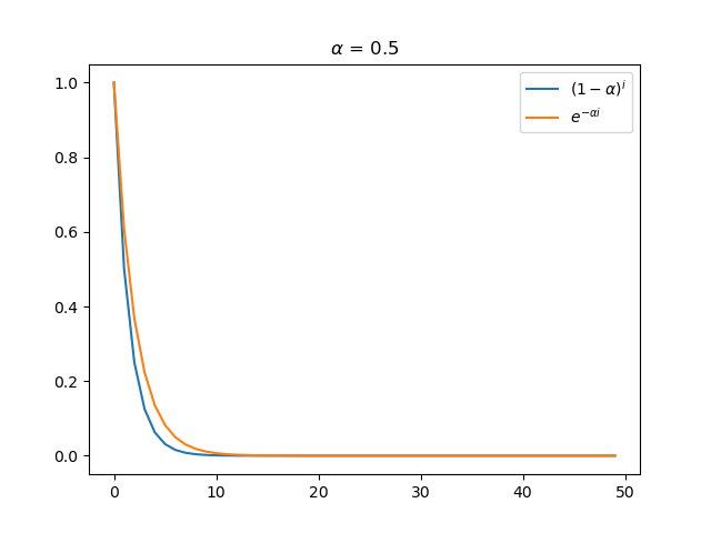
From the graphs, it is evident that the approximation is quite close, especially when \(\alpha\) is small.

Python codes:

import numpy as np
import matplotlib.pyplot as plt


alpha = 0.2
x = np.arange(0, 50)
y1 = [(1 - alpha)**i for i in x]
y2 = [np.exp(-alpha*i) for i in x]

plt.plot(x, y1, label = r'$(1-\alpha)^i$')
plt.plot(x, y2, label = r'$e^{-\alpha i}$')
plt.title(r'$\alpha$ = ' + str(alpha) )
plt.legend()
plt.show()

plt.figure()
alpha = 0.5
x = np.arange(0, 50)
y1 = [(1 - alpha)**i for i in x]
y2 = [np.exp(-alpha*i) for i in x]

plt.plot(x, y1, label = r'$(1-\alpha)^i$')
plt.plot(x, y2, label = r'$e^{-\alpha i}$')
plt.title(r'$\alpha$ = ' + str(alpha) )
plt.legend()
plt.show()

plt.figure()
alpha = 0.8
x = np.arange(0, 50)
y1 = [(1 - alpha)**i for i in x]
y2 = [np.exp(-alpha*i) for i in x]

plt.plot(x, y1, label = r'$(1-\alpha)^i$')
plt.plot(x, y2, label = r'$e^{-\alpha i}$')
plt.title(r'$\alpha$ = ' + str(alpha) )
plt.legend()
plt.show()