Pursuing the paper " cash-flow based dynamic inventory management"
This paper is written by Katehakis et al. (2016). Its main difference with Chao et al. (2008) and Gong et al. (2014) is its considering of non-stationary demand.
1. Problem description
Inventory-cash state \((x_n, y_n)\), where \(x_n\) the initial inventory in period $$n$, and $y_n$ denotes the amount of product that can be purchased using all the available cash $\gamma_n$ ($\gamma_n=cy_n$).
The cash flow fron inventory operations (\(D_n\) is the random demand):
\[\begin{aligned} R_n(D_n, q_n, x_n)=& p\min\{q_n+x_n, D_n\}-h(q_n+x_n-D_n)^+\\ =&p(q_n+x_n)-(p+h)(q_n+x_n-D_n)^+ \end{aligned}\]The cash flow from financial transactions is (\(i\) is deposite rate and \(l\) is bank loan interest rate):
\[\begin{aligned} K_n(q_n, y_n)=& c(y_n-q_n)[(1+i)\bf{1}_{\{q_n\leq y_n\}}+(1+l)\bf{1}_{\{q_n> y_n\}}] \end{aligned}\]State transition functions:
\[\begin{aligned} x_{n+1}=&(x_n+q_n-D_n)^+\\ y_{n+1}=&\left[R_n(D_n, q_n, x_n)+K_n(q_n, y_n)\right]/c \end{aligned}\]Optimality equation:
\[\begin{aligned} V_n(x_n, y_n)=&\sup_{q_n\geq 0} \mathbb{E}\left[V_{n+1}(x_{n+1},y_{n+1})\right]\\ =&\sup_{q_n\geq 0} \mathbb{E}\left[R_n(D_n, q_n, x_n)+K_n(q_n, y_n)\right] \end{aligned}\]2. The single period problem for period \(N\)
The expected net wealth at period \(N\) is:
\[G(x,q,y)=p(q+x)-(p-s)(q+x-D)^++c(y-q)[(1+i)\bf{1}_{\{q\leq y\}}+(1+l)\bf{1}_{\{q> y\}}]\]Lemma 1 \(G(x,q,y)\) is continuous and satisfies the following:
- It is concave in \(q\in [0, \infty]\).
- It is increasing and concave in \(x\), for \(s>0\).
- It is increasing and concave in \(y\), for all \(s<p\).
Proof
\[\frac{\partial G}{\partial q}=\begin{cases} p-c(1+i)-(p-s)F(q+x)\quad &q\leq y\\ p-c(1+l)-(p-s)F(q+x)& q>y \end{cases}\] \[\frac{\partial^2 G}{\partial q^2}=-(p-s)f(q+x)<0\]So, \(G(x,q,y)\) is concave in \(q\in [0,\infty]\).
When \(s>0\),
\[\frac{\partial G}{\partial x}=p-(p-s)F(q+x)>0\]So, \(G(x,q,y)\) is increasing and concave in \(x\), for \(s>0\).
\[\frac{\partial G}{\partial y}=c[(1+i)\bf{1}_{\{q\leq y\}}+(1+l)\bf{1}_{\{q> y\}}]>0\] \[\frac{\partial^2 G}{\partial y^2}=0\]So, \(G(x,q,y)\) is increasing and concave in \(y\).
□
Now we find the optimal ordering pattern for period \(N\) by drawing a picture of \(\partial G/\partial q\). Let \(p=5\), \(c=1\), \(i=0.01\), \(l=0.05\), \(s=2\), and Demand distribution \(\xi\sim N(10,2)\). The Matlab code:
function DrawPartialGq

p=3; c=2; i=0.01; l=0.1; s=1.5;
mu = 10; sigma = 2; % normaldistributiohn

x = 1; % initial inventory
partialGq1 = @(q)p - c * (1 + i) - (p - s) * normcdf(q + x, mu, sigma);
partialGq2 = @(q)p - c * (1 + l) - (p - s) * normcdf(q + x, mu, sigma);


fplot(@(x)0,[0, 20], '--', 'Linewidth', 2);
hold on;
fplot(partialGq1, [0, 20], 'r', 'Linewidth', 2);
fplot(partialGq2, [0, 20], 'b', 'Linewidth', 2);
xlabel({'$x+q$'}, 'Interpreter', 'latex');
legend({' ', '$q\leq y$', '$q>y$'}, 'Interpreter', 'latex');
hold off;
end
The picture:
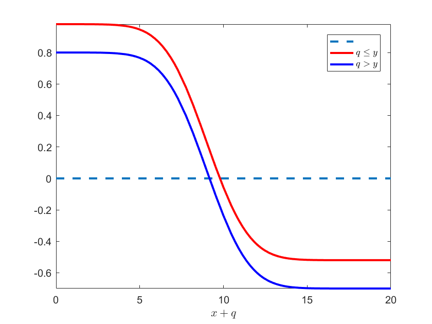
Since \(G(x,y,q)\) is continuous, we can conduct the optimal ordering policy below:
\[q^\ast=\begin{cases} (\alpha-x)^+\quad & x+y\leq \alpha\\ y & \alpha<x+y<\beta\\ (\beta-x)^+ & x+y\geq \beta \end{cases}\]Therefore, \(V_N(x,y)\) can be written to:
\[\begin{aligned} V_N(x,y)=&p(x+q^\ast)-(p+h)(x+q^\ast-D_N)^++K_n(q,y)\\ =&\begin{cases} px-(p+h)(x-D_N)^++cy(1+i) \quad &x>\beta\\ p\beta-(p+h)(\beta-D_N)^++c(x+y-\beta)(1+i)\quad &x\leq\beta, x+y\geq \beta\\ p(x+y)-(p+h)(x+y-D_N)^+ \quad&\alpha\leq x+y<\beta\\ p\alpha-(p+h)(\alpha-D_N)^+-(\alpha-x-y)(1+l)\quad & x+y<\alpha \end{cases}\end{aligned}\quad\tag{1}\]It can be easily shown that \(V_N(x,y)\) is jointly concave in \(x\) and \(y\).
2. The optimal ordering policy for period \(n<N\)
Theorem 1 for any \(n\), \(V_n(x,y)\) is jointly concave in \(x\) and \(y\).
Proof
Let \(z_n=x_n+q_n\),
\[V_n(x,y)=\max_{z\geq x} G_n(x,y,z)\\ G_n(x,y,z)=\mathbb{E}[V_{n+1}(x,y)]\]And the state transition function:
\[\begin{aligned} x_{n+1}&=(z_n-D_n)^+\\ c_{n+1}y_{n+1}&=p(z_n-D_n)-(p+h)(z_n-D_n)^++c(x_n+y_n-z_n)[(1+i)\bf{1}_{\{z_n\leq x_n+y_n\}}+(1+l)\bf{1}_{\{z_n> x_n+y_n\}}] \end{aligned}\]By recursion, we first prove for period \(n=N\). \(G_N(x,y,z)\) is apparenlty concave when \(n=N\). It can also be easily shown that \(V_N(x,y)\) is jointly concave in \(x\) and \(y\) from Eq. (1). Now we prove for period \(n<N\).
Assume \(V_{n+1}(x,y)\)$ is concave, the first derivatives of the state transition functions are the following:
\[\begin{cases} \frac{\partial x_{n+1}}{\partial z_n}&=1_{\{z_n\geq D_n\}}\\ \frac{\partial x_{n+1}}{\partial x_n}&=0\\ \frac{\partial x_{n+1}}{\partial y_n}&=0\\ \end{cases}\] \[\begin{cases} \frac{\partial y_{n+1}}{\partial z_n}&=p'-(p'+h')_{\{z_n>D_n\}}-c'_n(1+i)_{z_n\leq x_n+y_n}-c'_n(1+l)_{z_n\leq x_n+y_n}\\ \frac{\partial y_{n+1}}{\partial x_n}&=c'_n(1+i)_{z_n\leq x_n+y_n}+c'_n(1+l)_{z_n\leq x_n+y_n}\\ \frac{\partial y_{n+1}}{\partial y_n}&=c'_n(1+i)_{z_n\leq x_n+y_n}+c'_n(1+l)_{z_n\leq x_n+y_n}\\ \end{cases}\]The concavity is proved by the positive definiteness of Hessian matrix.
\[\begin{aligned} \frac{\partial G_n(x_n, y_n, z_n)}{\partial x_n }&=\mathbb{E}\left[\frac{\partial V_{n+1}(x_{n+1},y_{n+1})}{\partial x_{n+1}}\frac{\partial x_{n+1}}{\partial x_n}+\frac{\partial V_{n+1}(x_{n+1},y_{n+1})}{\partial y_{n+1}}\frac{\partial y_{n+1}}{\partial x_n}\right]\\ &=\mathbb{E}\left[\frac{\partial V_{n+1}(x_{n+1},y_{n+1})}{\partial y_{n+1}}\frac{\partial y_{n+1}}{\partial x_n}\right] \end{aligned}\] \[\begin{aligned} \frac{\partial G_n(x_n, y_n, z_n)}{\partial y_n }&=\mathbb{E}\left[\frac{\partial V_{n+1}(x_{n+1},y_{n+1})}{\partial x_{n+1}}\frac{\partial x_{n+1}}{\partial y_n}+\frac{\partial V_{n+1}(x_{n+1},y_{n+1})}{\partial y_{n+1}}\frac{\partial y_{n+1}}{\partial y_n}\right]\\ &=\mathbb{E}\left[\frac{\partial V_{n+1}(x_{n+1},y_{n+1})}{\partial y_{n+1}}\frac{\partial y_{n+1}}{\partial y_n}\right] \end{aligned}\] \[\begin{aligned} \frac{\partial G_n(x_n, y_n, z_n)}{\partial z_n }&=\mathbb{E}\left[\frac{\partial V_{n+1}(x_{n+1},y_{n+1})}{\partial x_{n+1}}\frac{\partial x_{n+1}}{\partial z_n}+\frac{\partial V_{n+1}(x_{n+1},y_{n+1})}{\partial y_{n+1}}\frac{\partial y_{n+1}}{\partial z_n}\right]\\ &=\mathbb{E}\left[\frac{\partial V_{n+1}(x_{n+1},y_{n+1})}{\partial y_{n+1}}\frac{\partial x_{n+1}}{\partial z_n}\right]+\mathbb{E}\left[\frac{\partial V_{n+1}(x_{n+1},y_{n+1})}{\partial y_{n+1}}\frac{\partial y_{n+1}}{\partial z_n}\right] \end{aligned}\]Very complex proof ! (adopt property “max of a compound concave function is also concave”)
Let \(\frac{\partial G_n(x_n, y_n, z_n)}{\partial z_n}=0\), optimal ordering policies for each period can be obtained. It is very similar to Eq. (1).
4. Myopic policy
4.1 Myopic policy I
Let
\[\underline{s}_n=\begin{cases} -h_n\qquad &n<N\\ s, & n=N \end{cases}\]And,
\[\begin{aligned} \underline{a}_n&=\frac{p_n-c_n(1+l_n)}{p_n-\underline{s}_n}\\ \underline{b}_n&=\frac{p_n-c_n(1+i_n)}{p_n-\underline{s}_n}\\ \underline{\alpha}_n&=F^{-1}_n(\underline{a}_n)\\ \underline{\beta}_n&=F^{-1}_n(\underline{b}_n) \end{aligned}\]Myopic policy I is shown by the following equation.
\[\underline{q}_n(x_n, y_n)= \begin{cases} (\underline{\beta}_n-x_n)^+, \quad &x_n+y_n\geq \beta_n\\ y_n, &\underline{\alpha}_n\leq x_n+y_n\leq \underline{\beta}_n\\ (\underline{\alpha}_n-x_n)^+, \quad &x_n+y_n< \alpha_n \end{cases}\]Theorem 2 for any \(n\), the optimal ordering controlling parameter:
\[\begin{aligned} \alpha_n\geq \underline{\alpha}_n\\ \beta_n\geq \underline{\beta}_n \end{aligned}\]Proof
Let \(\frac{\partial G_n(x_n, y_n, z_n)}{\partial z_n }=0\), we get
\[\mathbb{E}\left[\frac{\partial V_{n+1}(x_{n+1},y_{n+1})}{\partial y_{n+1}}\frac{\partial x_{n+1}}{\partial z_n}\right]+\mathbb{E}\left[\frac{\partial V_{n+1}(x_{n+1},y_{n+1})}{\partial y_{n+1}}\frac{\partial y_{n+1}}{\partial z_n}\right]=0\] \[\mathbb{E}\left[ \frac{\partial V_{n+1}}{\partial y_{n+1}}\left(\frac{\partial x_{n+1}}{\partial z_n}+\frac{\partial y_{n+1}}{\partial z_n}\right) \right]=0\]So, \(\alpha_n\) is the unique solution of
\[\mathbb{E}\left[ \frac{\partial V_{n+1}}{\partial y_{n+1}}\left(1_{\alpha_n>D_n}+p'-(p'+h')_{\{\alpha_n>D_n\}}-c'_n(1+l)\right) \right]=0\]That is
\[\mathbb{E}\left[ \frac{\partial V_{n+1}}{\partial y_{n+1}}\left(p'-(p'+h')_{\{\alpha_n>D_n\}}-c'_n(1+l)\right) \right]=-\mathbb{E}\left[\frac{\partial V_{n+1}}{\partial y_{n+1}}(1_{\alpha_n>D_n})\right]\]The right side is non-positive, so
\[\mathbb{E}\left[ \frac{\partial V_{n+1}}{\partial y_{n+1}}\left(p'-(p'+h')_{\{\alpha_n>D_n\}}-c'_n(1+l)\right) \right]\leq 0\]Because \(\frac{\partial V_{n+1}}{\partial y_{n+1}}\) is always non-negative,
\[\mathbb{E}\left[p'-(p'+h')_{\{\alpha_n>D_n\}}-c'_n(1+l)\right]\leq 0\]We can obtain:
\[F(\alpha_n)\geq \frac{p_n-c_n(1+l_n)}{p_n-s_n}\] Very lengthy and complex proofs afterwards...□
My major concern:
- In Lemma 2, why \(V_n(x_n, y_n)\) is increasing in \(x_n\) and \(y_n\)? the proof in the appendix does not prove this. (Suppose we have very high unit holding cost, increasing \(x_n\) would result in the decreasing of \(V\))
- In the appendix proof page 35, why “the second-order derivatives of \(x_{n+1}\) and \(y_{n+1}\)with respect to \(z_n\), \(x_n\) and \(y_n\) are all zero”? I think the second-order derivative of $x_{n+1}\(to\)z_n$$ is not zero. It is the probability distribution function of the stochastic demand, which is non-negative.
5. Numercial analysis
I code the stochastic dynamci programming algorithm for this problem, but my results is different from the author’s in Figure 2 of the paper. In addition, why the authors adopt the zero-inflated Poisson distribution? It is very uncommon distribution.
Enjoy Reading This Article?
Here are some more articles you might like to read next: